Why bent didgeridoos confuse our acoustic simulator - and a fix

A non-technical introduction

When we design a didgeridoo on the computer, we want the simulator to predict the pitches the real instrument will play. For a straight didgeridoo - a tapering tube - our simulator nails it: predicted pitches match measurements to within a few cents (a cent is 1/100 of a semitone - about the smallest pitch difference a trained ear can pick up).

The trouble starts when the instrument is bent. Many real didges are curved: some are coiled to be more portable, others follow the natural shape of a branch. Our fast simulator assumes the bore is straight, so when we feed it a bent didge it makes a systematic mistake: predicted pitches come out too low. On the seven didges we tested, the error averages 41 cents - almost half a semitone. That is well past “audible”; it is enough to send a maker chasing a tuning fault that does not actually exist in the instrument.

There is a slow simulator that gets the bent case right (it actually models the bend in 3D), but it is 100–1000× slower than the fast one. That matters because we use the fast simulator inside an evolutionary search loop that tries thousands of geometries - slow is not an option.

This post is about how we can keep the speed of the fast simulator while recovering most of the accuracy of the slow one, by applying a small analytical correction based on the geometry of the bend. On the seven test didges, this correction closes about two thirds of the cent gap - for basically no extra compute.

Two ways to simulate a didgeridoo

Before we can talk about the fix, here is what the two simulators actually do.

Transmission line modelling (TLM)

The transmission line model treats the didgeridoo as a sequence of short cylindrical or conical segments along a single axis. For each segment it applies the standard one-dimensional wave equation, then chains the segments together with the right boundary conditions. The simulator is essentially solving for the pressure response along an idealised straight tube whose diameter follows the actual bore.

This is the bore the TLM “sees” - a 1D profile along a perfectly straight axis:

TLM is extremely fast (milliseconds per impedance spectrum) and accurate as long as the underlying assumption holds: that the bore can be treated as a straight 1D waveguide.

3D Finite Element Modelling (FEM-3D)

The 3D FEM solver does something fundamentally different: it builds an actual tetrahedral mesh of the bore - in 3D space, along the real centerline of the bent instrument - and solves the 3D Helmholtz equation on that mesh directly. There is no “1D approximation” anywhere; the bend lives in the actual geometry the solver sees.

Here is the same arusha didgeridoo, swept along the bent centerline used by FEM-3D:

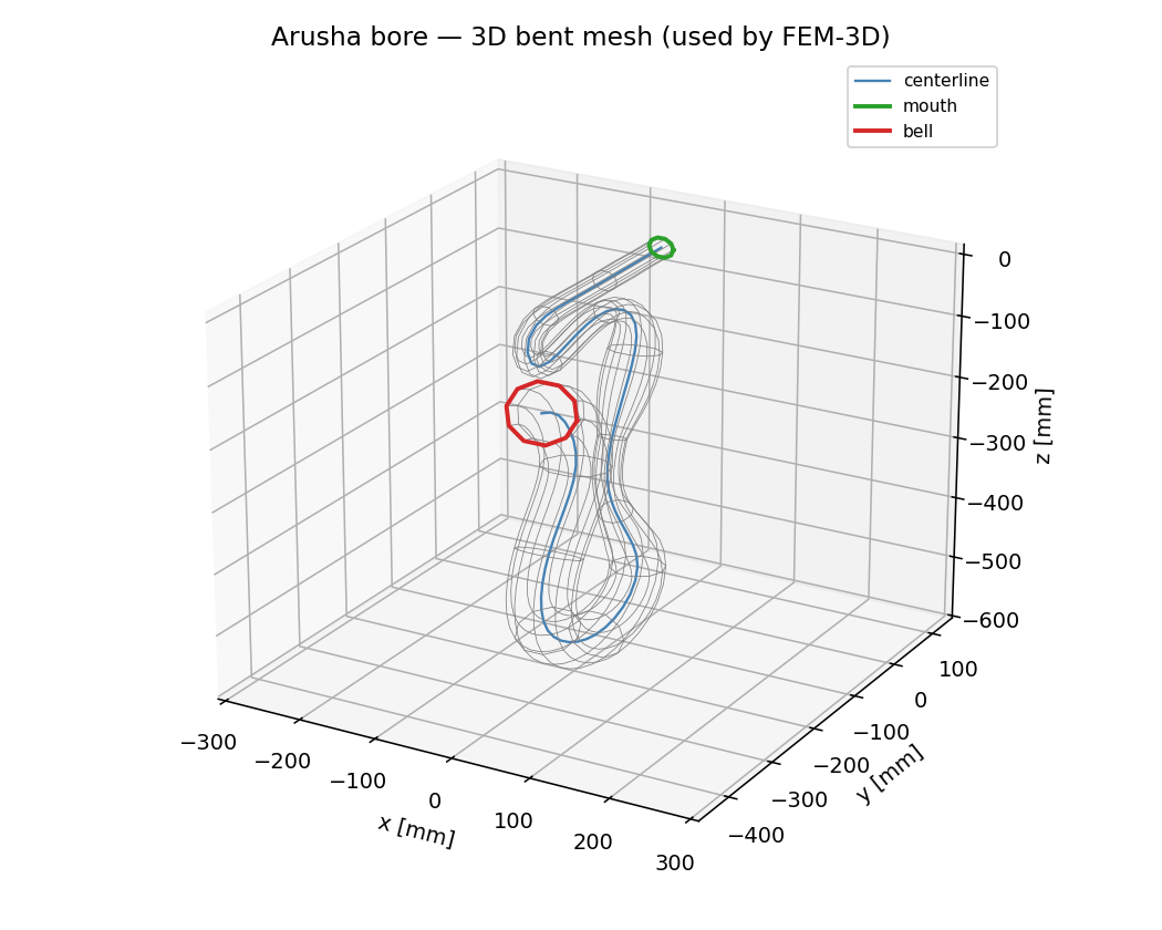
This is much more expensive (seconds per spectrum), but it is also the ground truth: when the bent didge is built and measured, FEM-3D’s predicted pitches match. The straight-axis TLM is the one that lands ~40 cents low.

The fix: shorten the bore along the inside of the bend

Why bent tubes sound higher

Imagine the wavefront of sound travelling along a curved tube. Along the inner edge of the bend the path is shorter than along the outer edge. The sound effectively “cuts the corner”. Because the resonance frequencies of a tube depend on its acoustic length, a curved tube behaves like a slightly shorter straight tube, and a shorter tube plays higher.

The amount of shortening depends on two local quantities at every point along the bore:

• the curvature $\kappa(s)$ of the centerline at position $s$ - i.e. how sharply it bends there;
• the bore radius $a(s)$ - fatter sections care more about being bent than narrow ones.

Both of these are something we already have: $\kappa(s)$ comes from the centerline curve we used to build the bent mesh, and $a(s)$ comes from the geo itself.

The correction in one formula

Curved-waveguide theory (Felix & Pagneux, among others) gives a closed-form expression for the leading-order frequency shift of the lowest acoustic mode in a toroidal duct. Translated into a per-segment length correction:

\[\mathrm{d}L_\mathrm{eff}(s) \;=\; \mathrm{d}s \,\Bigl(1 - \alpha\,\kappa(s)^2\,a(s)^2\Bigr)\]

where

• $s$ is the arc-length coordinate along the bent centerline, measured in millimetres from the mouthpiece ($s = 0$) to the bell ($s = L$, the total bore length).
• $\mathrm{d}s$ is an infinitesimal step along that centerline - the geometric length of a tiny segment of the real, curved bore.
• \(\mathrm{d}L_\mathrm{eff}(s)\) is the effective acoustic length of that same tiny segment, as seen by the 1D wave equation. This is the number we feed into TLM in place of $\mathrm{d}s$. Because the term in parentheses is less than one, \(\mathrm{d}L_\mathrm{eff} < \mathrm{d}s\) wherever the bore is bent - the acoustic tube is shorter than the physical tube.
• $\kappa(s)$ is the local curvature of the centerline at $s$, in units of $\mathrm{mm}^{-1}$. It is the reciprocal of the local bend radius: $\kappa = 1/R$. A straight section has $\kappa = 0$; a tightly coiled section has large $\kappa$.
• $a(s)$ is the local bore radius at $s$, in millimetres - half of the diameter from the geo at axial position $s$.
• $\alpha$ is a dimensionless proportionality constant of order one, set by curved-waveguide theory (see next subsection). It is the only free parameter of the correction.

The product $\kappa(s)\cdot a(s)$ is dimensionless - it is the ratio of bore radius to bend radius - so $\alpha\,\kappa^2 a^2$ is dimensionless too, and the formula respects units.

The recipe:

1. For each point along the bore, multiply the segment length $\mathrm{d}s$ by the local shortening factor $1 - \alpha\,\kappa^2 a^2$.
2. Integrate to get a corrected x-axis.
3. Feed the corrected geo - same diameters, shorter axis - back into the fast TLM.

That is it. No mesh, no 3D solve, no neural network. We are simply telling the 1D simulator “the effective tube is a little shorter than its arc length, and here is by how much”.

The $\alpha$ parameter

The quantity $\kappa\cdot a$ is dimensionless: it is the ratio of bore radius to radius of curvature. For a typical didgeridoo coiling that reaches a curvature of 1/0.2 m and a bore radius of 4 cm, $\kappa\,a \approx 0.2$ and $(\kappa a)^2 \approx 0.04$ - so the correction asks for about a 4 % shortening, locally, where the bend is tightest.

$\alpha$ is the proportionality constant in front. The theoretical value from the toroidal-mode analysis is

\[\alpha = \tfrac{1}{4}\]

We treat $\alpha$ as a parameter and check the theory empirically. If the data picks out $\alpha = 0.25$ on its own, that is a satisfying confirmation that the physics is what we think it is.

The experiment

We took seven didges from the Didgitaldoo archive - arusha, malveira, open-didgeridoo, matema, nazare, tamaki1, kizimkazi - and ran each of them through:

1. Bare TLM (straight, fast).
2. Corrected TLM with $\alpha \in {0.10,\ 0.25,\ 0.50,\ 1.00}$.
3. FEM-3D on the bent mesh (slow ground truth).

For each simulation we extracted the first five impedance peaks. We then matched bare-TLM and corrected-TLM peaks to FEM-3D peaks using nearest- log-frequency, ignoring matches that were farther than 200 cents apart (those are not really the same mode and would confuse the statistics).

Headline numbers

$\alpha$	mean |residual|	fraction of shift recovered
0.10	31.3 cents	27 %
0.25	14.4 cents	66 %
0.50	20.3 cents	52 %
1.00	85.5 cents	−101 % (worse than no correction)

The starting point - bare TLM vs FEM-3D - was a mean cent error of about 41 cents. With the analytical correction at $\alpha = 0.25$, the mean error drops to roughly 13 cents, recovering about two thirds of the shift. And the theory’s predicted $\alpha = 1/4$ is exactly the value the data picks out on its own - a nice confirmation that this really is the right leading-order physics.

What this looks like per mode

For each of the seven didges, the chart below compares the raw cent error (red, FEM-3D vs bare TLM) against the residual cent error after applying the analytical correction (orange, FEM-3D vs corrected TLM):

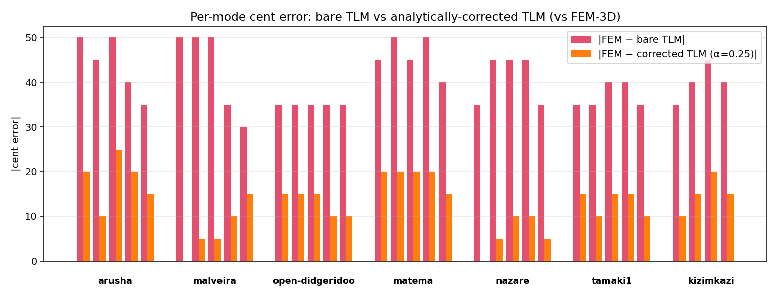
For every single mode of every single didge, the corrected bar is shorter than the bare bar. The remaining residual is typically the higher modes of the more aggressively bent geos - exactly where the leading-order $(\kappa a)^2$ scaling is expected to start missing terms.

What this looks like as a spectrum

Here is the impedance spectrum of arusha (the didge in the bore-image figures above), comparing all three simulators on the same min-max axis:

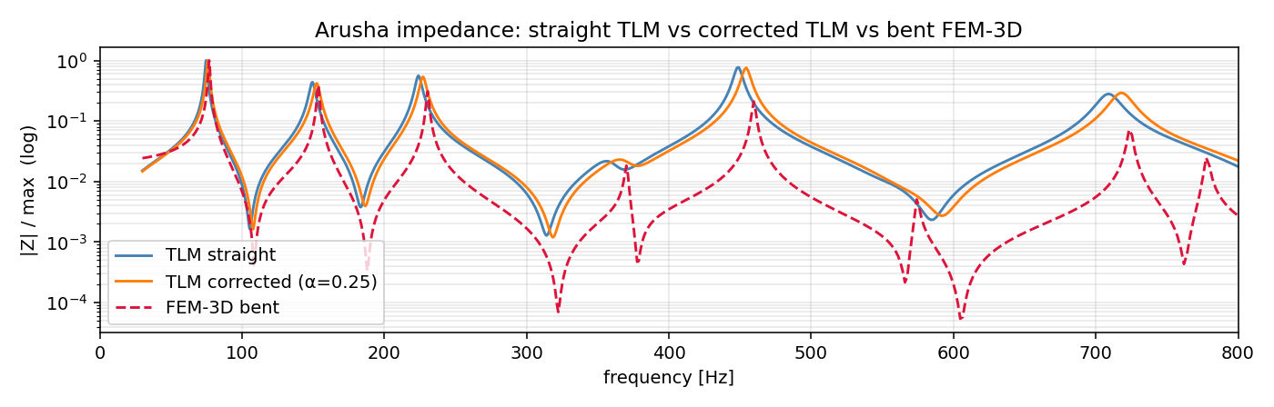
The blue (bare TLM) peaks sit visibly left of the red dashed (FEM-3D) peaks - that is the cent error. The orange (corrected TLM) peaks land closer to the FEM-3D peaks, especially at low frequencies where the fundamental and the first few overtones are.

Caveats

A few honest ones:

• The correction is leading-order in $(\kappa a)$. Higher modes - whose wavelengths are short enough that they “feel” the cross-section structure of the bend, not just the centerline curvature - are improved but not perfected.
• We are post-processing the geometry, not the spectrum. Peak amplitudes and bandwidths are not corrected - only peak positions. If you care about timbre and not just pitch, this method is not enough on its own.
• Seven didges is more of a unit test than a real validation. The next step is to run the same comparison on a much larger parameterised family of geometries to confirm $\alpha = 0.25$ holds across the design space.

Speed

The corrected TLM runs in essentially the same time as bare TLM: building the corrected geo is a single $O(N)$ trapezoidal integral over the centerline. We pay milliseconds for the correction itself, and the TLM solve afterwards is the usual milliseconds. So we keep the 100–1000× speedup over FEM-3D, and we recover about two thirds of the accuracy gap.

That is a very cheap correction for a very large quality improvement - exactly the trade-off our evolutionary geometry search needs.